Giving a Network Memory with a Recurrent Neural Network
In the three-triangles post, a multi-layer perceptron took a point (x, y) and decided whether it fell inside any of three triangles. Every network so far — the perceptron, the XOR MLP, the triangles — has taken one static input, all of it at once, and produced one answer.
Real data often does not arrive that way. A sentence is one word after another. A melody is one note after another. The input is a sequence in time, and each piece only makes sense in the context of what came before. To handle that, a network needs something none of our earlier ones had: memory.
This post builds the simplest network with memory — a recurrent neural network — from scratch in NumPy, and teaches it a tiny sequence.
The idea
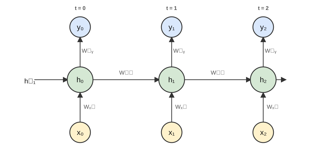
The trick is a hidden state that the network feeds back into itself. Call it . At each timestep the network reads the current input and the previous hidden state , mixes them, and produces a new hidden state . That new state carries forward to the next step. The hidden state is the memory.
A single timestep comes down to two equations:
The first line is the memory update: a weighted sum of the new input (through ) and the old state (through ), squashed by . The second line reads an output off the hidden state. Softmax over turns it into a probability for each possible next symbol.
What makes it recurrent is that the same weights , , are used at every timestep. There are no separate parameters for “the third word.” One set of parameters gets applied over and over as the sequence rolls past. The hero diagram at the top shows this unrolled: three copies of the same cell, threaded together by the hidden state, all sharing one set of weights.
The data
The toy problem is the “hello world” of sequences: learn the cyclic pattern a → b → c → a. Given a character, predict the next one, where c wraps back to a. If the network truly learns it, then feeding its own predictions back in should make it cycle a, b, c, a, b, c, … forever.
Three characters, so we one-hot encode each as a length-3 vector:
import numpy as np
import numpy.typing as npt

chars = ["a", "b", "c"]
vocab_size = len(chars)
char_to_ix = {ch: i for i, ch in enumerate(chars)}

# The sequence "abc": input "abc" should predict the next char "bca".
inputs_ix = [char_to_ix[c] for c in "abc"]
targets_ix = [char_to_ix[c] for c in "bca"]


def one_hot(ix: int) -> npt.NDArray[np.float64]:
    v = np.zeros((1, vocab_size), dtype=np.float64)
    v[0, ix] = 1.0
    return v
So input a ([1,0,0]) should predict b, input b should predict c, and input c should predict a. That last wrap-around is the whole point. The only way to know that c is followed by a and a is followed by b is to remember where in the cycle we are. That memory lives in .
The network
The network holds three weight matrices and two biases:
hidden_size = 8
learning_rate = 0.1
epochs = 2000

rng = np.random.default_rng(1)
w_xh = rng.standard_normal((vocab_size, hidden_size)) * 0.1   # input  -> hidden
w_hh = rng.standard_normal((hidden_size, hidden_size)) * 0.1  # hidden -> hidden
w_hy = rng.standard_normal((hidden_size, vocab_size)) * 0.1   # hidden -> output
b_h = np.zeros((1, hidden_size))
b_y = np.zeros((1, vocab_size))
As in the XOR post, the weights start as small random numbers rather than zeros. If every weight were identical, all eight hidden units would compute the same value, receive the same gradient, and update in lockstep forever — the symmetry problem. Small random init breaks that so the hidden units can specialise. Scaling by 0.1 keeps them small, which matters later when we look at what backpropagation does to gradients over many steps.
We also need softmax to turn the output scores into probabilities:
def softmax(x: npt.NDArray[np.float64]) -> npt.NDArray[np.float64]:
    e = np.exp(x - np.max(x))
    return e / np.sum(e)
Forward pass
The forward pass walks the sequence one step at a time, carrying forward. We stash every intermediate value in a dictionary keyed by timestep, because backpropagation will need all of them:
hs = {-1: np.zeros((1, hidden_size))}  # h_{-1}: memory starts empty
xs, ps = {}, {}
loss = 0.0

for t in range(len(inputs_ix)):
    xs[t] = one_hot(inputs_ix[t])
    hs[t] = np.tanh(xs[t] @ w_xh + hs[t - 1] @ w_hh + b_h)
    y = hs[t] @ w_hy + b_y
    ps[t] = softmax(y)
    loss += -np.log(ps[t][0, targets_ix[t]])
hs[-1] starts as all zeros: before the sequence begins, the network remembers nothing. And hs[t] depends on hs[t - 1], which depends on hs[t - 2], and so on. The hidden states form a chain reaching all the way back to the start. That chain is what backpropagation will have to unwind.
The loss is cross-entropy: at each step we look up the probability the network assigned to the correct next character and add its negative log. Confident and right, is near zero. Confident and wrong, the penalty is large.
Backpropagation through time
This is the heart of the post. In the MLP, backpropagation pushed error backward through layers. In an RNN the same weights are reused at every timestep, so we push error backward through time instead, and every timestep contributes to the gradient of that one shared set of weights. This is backpropagation through time (BPTT).
Because , , appear at every step, the total gradient of each is a sum over all timesteps:
Let us derive each piece. Start at the output. It is the easy part, because it is local to each step. For a softmax followed by cross-entropy, the gradient of the loss with respect to the pre-softmax scores is the one clean result everyone remembers: predicted probabilities minus the one-hot target.
Call that . From it the output weights follow directly, since :
Now the hard part: the hidden state. The gradient arriving at has two sources, and that split is the whole idea of BPTT. One is the output at the same timestep, through . The other is the next hidden state , because was fed forward into it. So the total gradient at is:
That second term is why we walk backward through time. To know the gradient at , we must already have the gradient at . Call the incoming future term and let be the full sum above.
Next we pass back through the . Since and the derivative of is , the gradient with respect to the pre-activation is:
where is elementwise multiplication. From every weight in the update falls out, exactly as in the MLP — one term added into the running sum for this timestep:
Finally, the chain link that carries error into the past. Since enters through , the gradient handed back to the previous step is:
Read that last line closely, because it is the villain of the sequel. Every step backward multiplies the gradient by again. Hold that thought.
In code, the backward pass is the derivation transcribed line for line. We initialise the gradient accumulators to zero and the “future” gradient to zero (there is no timestep after the last one), then loop backward:
dw_xh = np.zeros_like(w_xh)
dw_hh = np.zeros_like(w_hh)
dw_hy = np.zeros_like(w_hy)
db_h = np.zeros_like(b_h)
db_y = np.zeros_like(b_y)
dh_next = np.zeros((1, hidden_size))

for t in reversed(range(len(inputs_ix))):
    dy = ps[t].copy()
    dy[0, targets_ix[t]] -= 1.0        # p_t - one_hot(target)

    dw_hy += hs[t].T @ dy              # output weights, summed over t
    db_y += dy

    dh = dy @ w_hy.T + dh_next          # error from this output + from the future
    dh_raw = (1.0 - hs[t] ** 2) * dh    # back through tanh

    db_h += dh_raw
    dw_xh += xs[t].T @ dh_raw           # input->hidden, summed over t
    dw_hh += hs[t - 1].T @ dh_raw       # hidden->hidden, summed over t

    dh_next = dh_raw @ w_hh.T           # hand the gradient to the previous step
Notice how every weight gradient uses +=, not =: each timestep adds its contribution to the shared total. That summation is weight sharing seen from the gradient’s side.
One practical safeguard before the update: gradient clipping. Recurrent gradients can occasionally blow up, so we cap their magnitude, then take a plain gradient-descent step:
for d in (dw_xh, dw_hh, dw_hy, db_h, db_y):
    np.clip(d, -5, 5, out=d)

w_xh -= learning_rate * dw_xh
w_hh -= learning_rate * dw_hh
w_hy -= learning_rate * dw_hy
b_h -= learning_rate * db_h
b_y -= learning_rate * db_y
Trying it out
Wrap the forward and backward passes in a training loop over the 2000 epochs, printing the loss now and then. Running it:
epoch    0  loss 3.3021
epoch  400  loss 0.0071
epoch  800  loss 0.0033
epoch 1200  loss 0.0022
epoch 1600  loss 0.0016
The loss starts near , which is three characters at chance ( each), and collapses toward zero. The network has memorised the transitions.
The real test is sampling: seed it with one character, then feed each prediction back in as the next input and let it run on its own.
def sample(seed_ix: int, n: int) -> str:
    h = np.zeros((1, hidden_size))
    ix = seed_ix
    out = [chars[ix]]
    for _ in range(n):
        x = one_hot(ix)
        h = np.tanh(x @ w_xh + h @ w_hh + b_h)
        p = softmax(h @ w_hy + b_y)
        ix = int(np.argmax(p))
        out.append(chars[ix])
    return "".join(out)


print("sample:", sample(char_to_ix["a"], 8))
The output:
sample: abcabcabcStarting from a, the network cycles a, b, c, a, b, c, … indefinitely, driving itself off nothing but its own hidden state. It learned more than “which character follows which.” It learned the loop, including the wrap where c returns to a, and that is only possible because the hidden state remembers where in the cycle it is.
The wall: memory that fades
We just taught an RNN a three-step cycle and it nailed it. Now push on the thing that makes RNNs famous, and famously limited. Make the dependency long-range: suppose the character the network must predict now depends on one it saw many steps ago. Can a plain RNN carry information that far?
Look again at the one line from the derivation I flagged:
To send a gradient from timestep back to a timestep steps earlier, we pass through that link times, and each pass multiplies the gradient by (roughly) . Over steps that is raised to the -th power. Multiply by a matrix whose entries are small, again and again, and the product races toward zero. Here is that exact product, using our small-initialised :
grad = np.eye(hidden_size)
for k in range(1, 26):
    grad = grad @ w_hh
    if k in (1, 5, 10, 20, 25):
        print(f"after {k:>2} steps: gradient norm = {np.linalg.norm(grad):.2e}")
after 1 steps: gradient norm = 7.34e-01
after 5 steps: gradient norm = 1.93e-03
after 10 steps: gradient norm = 1.14e-06
after 20 steps: gradient norm = 5.68e-13
after 25 steps: gradient norm = 3.99e-16The gradient does not just shrink, it evaporates. Twenty steps back it is around ; by twenty-five it has hit numerical zero. This is the vanishing gradient problem. A number that small carries no usable signal, so during training the weights get told essentially nothing about how events far in the past should affect the present. Our three-character cycle is short enough to learn without trouble, but a dependency stretching across dozens of steps never gets learned. The error signal cannot reach that far back. (Push the other way, toward larger values, and the same repeated multiplication makes gradients explode instead. That is why we clipped them.)
The root cause is structural. A plain RNN overwrites its entire hidden state at every step with a fresh , so old information is squeezed and re-squeezed until nothing survives. The network has no way to hold a value untouched across many steps.
That is exactly the problem the LSTM was invented to solve. It adds a separate cell state that runs straight through the timesteps with only light, additive edits, plus gates that learn when to write to it, when to erase it, and when to read from it. The result is a memory the network can protect across long spans instead of clobbering it every step. That is the next post.
Complete code
Here is the whole thing in one file:
import numpy as np
import numpy.typing as npt

chars = ["a", "b", "c"]
vocab_size = len(chars)
char_to_ix = {ch: i for i, ch in enumerate(chars)}

inputs_ix = [char_to_ix[c] for c in "abc"]
targets_ix = [char_to_ix[c] for c in "bca"]


def one_hot(ix: int) -> npt.NDArray[np.float64]:
    v = np.zeros((1, vocab_size), dtype=np.float64)
    v[0, ix] = 1.0
    return v


hidden_size = 8
learning_rate = 0.1
epochs = 2000

rng = np.random.default_rng(1)
w_xh = rng.standard_normal((vocab_size, hidden_size)) * 0.1
w_hh = rng.standard_normal((hidden_size, hidden_size)) * 0.1
w_hy = rng.standard_normal((hidden_size, vocab_size)) * 0.1
b_h = np.zeros((1, hidden_size))
b_y = np.zeros((1, vocab_size))


def softmax(x: npt.NDArray[np.float64]) -> npt.NDArray[np.float64]:
    e = np.exp(x - np.max(x))
    return e / np.sum(e)


def train() -> None:
    global w_xh, w_hh, w_hy, b_h, b_y
    for epoch in range(epochs):
        hs = {-1: np.zeros((1, hidden_size))}
        xs, ps = {}, {}
        loss = 0.0

        # forward pass over the sequence
        for t in range(len(inputs_ix)):
            xs[t] = one_hot(inputs_ix[t])
            hs[t] = np.tanh(xs[t] @ w_xh + hs[t - 1] @ w_hh + b_h)
            y = hs[t] @ w_hy + b_y
            ps[t] = softmax(y)
            loss += -np.log(ps[t][0, targets_ix[t]])

        # backward pass through time
        dw_xh = np.zeros_like(w_xh)
        dw_hh = np.zeros_like(w_hh)
        dw_hy = np.zeros_like(w_hy)
        db_h = np.zeros_like(b_h)
        db_y = np.zeros_like(b_y)
        dh_next = np.zeros((1, hidden_size))

        for t in reversed(range(len(inputs_ix))):
            dy = ps[t].copy()
            dy[0, targets_ix[t]] -= 1.0

            dw_hy += hs[t].T @ dy
            db_y += dy

            dh = dy @ w_hy.T + dh_next
            dh_raw = (1.0 - hs[t] ** 2) * dh

            db_h += dh_raw
            dw_xh += xs[t].T @ dh_raw
            dw_hh += hs[t - 1].T @ dh_raw

            dh_next = dh_raw @ w_hh.T

        for d in (dw_xh, dw_hh, dw_hy, db_h, db_y):
            np.clip(d, -5, 5, out=d)

        w_xh -= learning_rate * dw_xh
        w_hh -= learning_rate * dw_hh
        w_hy -= learning_rate * dw_hy
        b_h -= learning_rate * db_h
        b_y -= learning_rate * db_y

        if epoch % 400 == 0:
            print(f"epoch {epoch:>4}  loss {loss:.4f}")


def sample(seed_ix: int, n: int) -> str:
    h = np.zeros((1, hidden_size))
    ix = seed_ix
    out = [chars[ix]]
    for _ in range(n):
        x = one_hot(ix)
        h = np.tanh(x @ w_xh + h @ w_hh + b_h)
        p = softmax(h @ w_hy + b_y)
        ix = int(np.argmax(p))
        out.append(chars[ix])
    return "".join(out)


train()
print("sample:", sample(char_to_ix["a"], 8))