RAG and vector retrieval

You would have seen YouTube videos titled “Is Retrieval-augmented generation dead?”, once when context windows reached a million tokens, and once when agentic search arrived and models started grepping their way through code repositories. Neither killed it. What both did kill is the 2023 shape of it: chunk at 512 tokens, embed, take the top five by cosine similarity, paste into the prompt, hope.

That pipeline is still the one most tutorials teach, and it is the one that gets to 70% on a demo and stalls there forever. This article is about what replaces it, and about the decision that comes before any of it - whether you should be retrieving at all.

First, decide whether you need retrieval

Retrieval is machinery you have to build, evaluate, secure and keep in sync with a changing corpus. Before you take that on, check whether the problem needs it.

If the whole corpus fits in the context window, put it there. With a 1M-token context and prompt caching, a corpus under a few hundred thousand tokens - an internal handbook, a product spec, a year of policy documents, the full text of a contract set - is better handled by loading all of it and caching the prefix. No chunking decisions, no recall ceiling, no index to keep fresh. The model sees every word.

Token counts are hard to feel, so let’s do some rough calculations. English runs about 1.3 tokens per word, and a single-spaced A4 page at 12 pt with normal margins holds roughly 550 words:

$$\begin{aligned} \text{one page} \;&\approx\; 1.3 \times 550 &&\approx\; 700 \text{ tokens} \cr \text{a 1M window} \;&\approx\; 10^6 / 700 &&\approx\; 1{,}400 \text{ pages, or } 750{,}000 \text{ words} \cr \text{usable for corpus} \;&\approx\; (200{,}000 \times \tfrac{2}{3}) / 700 &&\approx\; 190 \text{ pages} \end{aligned}$$

That third line is the one to design against, and it comes from two separate limits. Do not plan to fill the window: answer quality degrades as the context fills, well before the hard limit, so treat 200K tokens as the band where responses stay sharp whatever the model advertises. And the corpus does not get all of even that - the same context holds the system prompt, every turn of the conversation so far, the model’s thinking (echoed back into the history on each following turn, on models where adaptive thinking is on by default) and the answer being written. Thirty turns at 1,500 tokens of reply and reasoning is another 45,000 tokens, and running out is a hard error rather than a graceful degradation, so give the corpus at most two thirds. The symptom of ignoring this is a chat that answers the first question well and drifts wrong a few turns later.

For scale, 190 pages is a substantial employee handbook or a folder of contracts. While making model API calls, order the request so the corpus sits in the cached prefix and the conversation accumulates after the last cache breakpoint, so the part that grows every turn never invalidates the part you paid to cache; if a long chat does approach the window, server-side compaction will summarise earlier context. Only compact conversation turns and not the corpus.

The cost can work out better than expected. On Claude Opus 4.5 at $5 per million input tokens, a 200,000-token corpus costs $1.00 to send uncached - and $1.25 on the first query if you cache it, since a cache write runs about 1.25× the base rate. Every query after that is $0.10, because a cached read is a tenth of base. A retrieval pipeline that pulls twelve chunks of 600 tokens sends 7,200 uncached tokens, about $0.036. Setting those equal - with $C$ the corpus size in tokens, and $0.50 per million (the $5 base rate at the cached tenth) on the left - gives the crossover:

$$\begin{aligned} \underbrace{0.50}_{\text{cached rate per M}} \times \frac{C}{10^6} &= \underbrace{0.036}_{\text{one RAG query}} \cr C &\approx 72{,}000 \text{ tokens} \end{aligned}$$

So on marginal token cost alone, retrieval starts winning at around 70k tokens of corpus. But that comparison ignores everything else: the index store, the evaluation set. Fold in a few thousand dollars of engineering and a vector store to run, and the honest crossover is much further out. I recommend not building a retrieval stack for a corpus that fits inside the 190-page budget above unless something else really warrants it.

One caveats though. That write premium is not a one-off, because the default cache lifetime is five minutes, with a one-hour option. At low query volume you pay for the write repeatedly and the economics invert: ten queries an hour against a 200k-token cached prefix means one $1.25 write amortised over ten queries, which is worse per query than retrieving.

If the data is structured, query it. A question like “which three regions missed quota last quarter” is a GROUP BY, not a similarity search. Give the model a SQL tool and a schema.

If the corpus is a codebase, try search before embeddings. This is the one that has genuinely shifted. Code is full of exact identifiers, and an agent that can run grep, follow imports and read files usually beats a vector index over code chunks in small codebases - because the queries that matter are where is this symbol defined and what calls this, both of which are exact-match problems that embeddings actively blur.

Retrieval earns its place when the corpus is large, mostly prose, changes often, needs per-user access control, or has to produce citations that point at a source of record. That is a big class of problems. The rest of this article is about doing it properly.

The mental model: a cascade, not a lookup

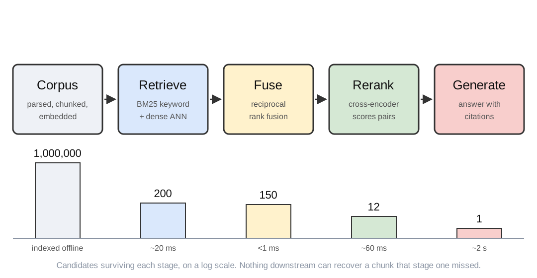
The single most useful reframe is that retrieval is a cascade of filters with widening cost and narrowing output, not a single lookup. Each stage is allowed to be sloppier than the next because it hands on fewer candidates.

• Stage 1 is cheap and wide. It scans a million chunks and returns a couple of hundred. Its only job is recall: get the right chunk into the candidate set.
• Stage 2 is expensive and narrow. It scores a couple of hundred query-document pairs properly and returns a dozen. Its job is precision: order them so the right one is at the top.
• Stage 3 is the model, which reads the dozen and writes the answer.

From this falls the one inequality that should govern how you spend your time. Let $R@n$ be the probability that the supporting passage is in the $n$ candidates stage 1 returns. Then end-to-end answer accuracy is bounded:

$$\text{Accuracy} \le R@n$$

Nothing downstream can recover a chunk stage 1 missed. A better reranker cannot promote a document that is not in the list. A better model cannot cite text it never saw. If your recall@100 is 0.85, you are working under a hard 85% ceiling and no amount of prompt engineering will move it.

This is why the first number you should measure is recall at the candidate count you actually use, and why almost every “our RAG is only 70% accurate” investigation ends in the same place: not the model, not the reranker, the chunk was never retrieved. Often it was never even indexed correctly, which brings us to the stage nobody writes about - messy, and entirely dependent on the source corpus format.

Stage zero: parsing is where most projects actually fail

Before a single embedding is computed, your documents have to become text. For plain Markdown this is free. For the PDFs, scanned forms, slide decks and spreadsheets that make up most real corpora, it is the hardest part of the project.

The failure mode is specific and quiet. A naive PDF text extractor reads a two-column page in the wrong order, so sentences interleave into nonsense. It flattens a table into a run of numbers with no column headers, so the row “Thailand | 2023 | 18.2%” becomes “Thailand 2023 18.2%” next to forty other stripped rows. It drops the header that said the units were millions. None of this raises an error. It produces text, the text gets embedded, and the embedding vector for a passage has lost the facts.

The test is simple: extract your text, then try to answer twenty of your own questions using nothing but Ctrl-F over the extracted text. If you cannot, no embedding model will. Do this before you choose a vector database.

What to reach for, in escalating order of cost:

• Native text extraction for PDFs with simple layout.
• A layout-aware parser - Docling, Marker, Unstructured - which recovers reading order, headings and table structure into Markdown or HTML.
• A vision model over the page images for anything scanned, handwritten, or heavy on diagrams. This is now cheap enough to be the default for hard documents rather than the last resort.

Extract into a format that can hold a hierarchy. Plain text is the wrong target. Documents are trees - sections contain subsections, tables contain rows which contain cells, lists nest inside list items - and flattening that into a line-by-line string destroys the nesting permanently. Extract to Markdown, or to an XML-shaped format such as HTML, so the structure/nesting survives as #/## levels or as <section>, <table> and <li>.

Markdown is the default: compact, cheap in tokens, and models read it natively. Switch to HTML where the nesting is real and Markdown turns ambiguous - merged-cell tables, clauses with three levels of numbered sub-clauses, forms with repeated groups. Either way the payoff is downstream: chunking on section boundaries and being able to hand back a whole parent section rather than a fragment of one.

Two things to preserve while you parse, because they are almost free at this stage and impossible to reconstruct later:

Structure. Keep headings as headings. The heading path of a chunk (Employee Handbook > Leave > Parental leave > Eligibility) is the single most useful piece of metadata you will have, both as a retrieval signal and as something to show the user.

Provenance. Every chunk should carry the document id, the page or section, and a character range. You need this for citations, for access control, for debugging, and for the moment someone asks where a number came from.

Chunking

Chunking exists for two independent reasons, and they are worth separating because only one of them is negotiable.

The hard limit: you cannot exceed the model’s maximum sequence length. Every embedding model has one. The classic BERT-based encoders cap at 512 tokens; several current models take 8,192 or more. What happens when you go over is implementation-specific and worth knowing before you find out in production: most local libraries and several hosted APIs truncate silently, handing back a perfectly valid-looking vector computed from only the first 512 tokens of your 2,000-token chunk, while others reject the request outright. Silent truncation is the dangerous one. Look up your model’s limit, and test which of the two behaviours you get.

The soft limit: even well under the maximum, a longer chunk is a worse chunk. A 1024-dimensional vector has a fixed capacity no matter how much text you feed it, so the more you put in, the fainter its representation of any particular fact inside becomes. A chunk covering three topics produces a vector that sits between all three and is the nearest neighbour of none of them.

The first sets a ceiling you must not cross. The second is that a chunk should hold information about one tightly related topic.

Practical defaults:

• 300 to 800 tokens. Below that you lose the referent; above it you dilute.
• Split on structure first, size second. Break at headings, then at paragraphs, and only fall back to a fixed window inside a section that is too long. A chunk that straddles two sections is worse than two uneven chunks.
• 10-15% overlap, so a fact that lands on a boundary appears whole somewhere.
• Never split a table. Keep it intact, and repeat the header row if you must break it.

The isolation problem

The deeper issue is not size. It is that a chunk lifted out of its document loses the things the document established once, at the top, and never repeated.

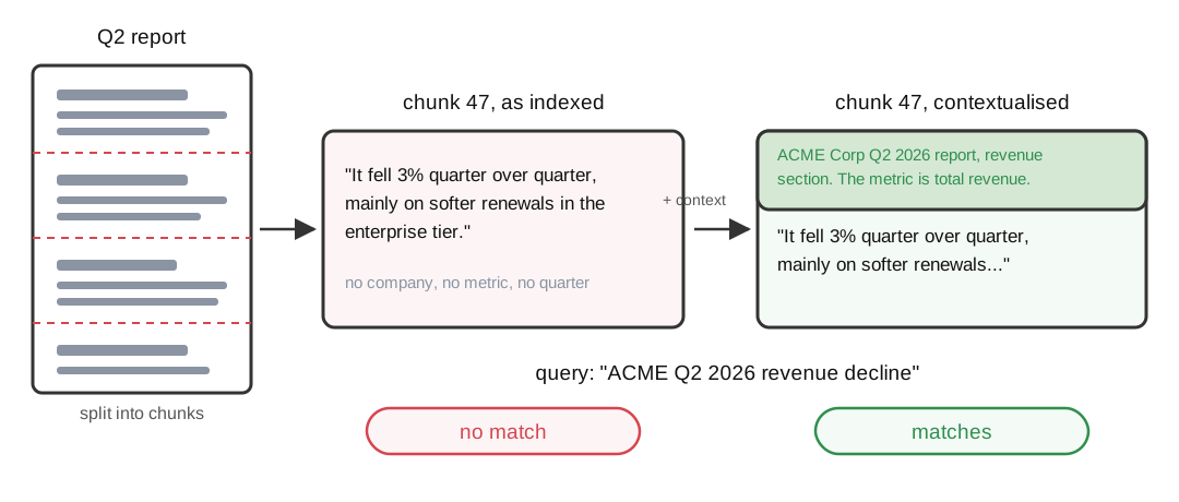
The chunk is a perfectly good sentence and a useless index entry. “It” is doing all the work, and the referent is nine paragraphs up.

The fix that works is contextual retrieval: before embedding, ask a cheap model to write a one- or two-sentence situating description of the chunk given the whole document, and prepend that to the chunk text you index. The full document goes in the prompt once and is cached; each chunk is a short completion against that cached prefix.

import anthropic

client = anthropic.Anthropic()

PROMPT = """Here is a chunk from the document above:

<chunk>
{chunk}
</chunk>

Write one or two short sentences situating this chunk within the document,
so that it can be found by search on its own. Name the entities, the metric,
the time period and the section that the chunk refers to only implicitly.
Output the sentences and nothing else."""


def contextualise(document: str, chunk: str) -> str:
    response = client.messages.create(
        model="claude-haiku-4-5",
        max_tokens=200,
        system=[
            {
                "type": "text",
                "text": f"<document>\n{document}\n</document>",
                # cached once per document, then read by every chunk of it
                "cache_control": {"type": "ephemeral"},
            }
        ],
        messages=[{"role": "user", "content": PROMPT.format(chunk=chunk)}],
    )
    return response.content[0].text.strip()


def index_document(document: str, chunks: list[str]) -> list[str]:
    # Process a document's chunks back to back: the cache TTL is five minutes,
    # and a cold cache turns a cheap read into a full-price write.
    return [f"{contextualise(document, c)}\n\n{c}" for c in chunks]

The economics are the reason this is now standard rather than exotic. Take a 10,000-token document chunked into roughly seventeen pieces, on Claude Haiku 4.5 at $1 per million input and $5 per million output:

Line	Tokens	Rate	Cost
Cache write, once per document	10,000	$1.25/M	$0.0125
Cache reads, 16 further chunks	160,000	$0.10/M	$0.0160
Output, 17 × 70 tokens	1,190	$5.00/M	$0.0060
Per 10,000-token document			$0.035

That is about $3.50 per million tokens of corpus, one-time. For a 100M-token corpus, $350 to remove a whole category of retrieval failure. Note the ordering constraint in the code comment - if you interleave documents, every chunk pays the write rate instead of the read rate - 12.5× more per input token, which roughly sextuples the bill for the document.

Two cheaper variants, worth knowing:

Heading-path prefixing. Prepend the structural breadcrumb you already captured at parse time. Free, no model call, and it recovers a surprising fraction of the same benefit on well-structured documents. Do this even if you also do contextual retrieval.

Small-to-big. Embed the small chunk but return it and its parent section to the model. Retrieval stays sharp; the model gets enough surrounding text to reason. This composes with everything else and costs nothing.

Embeddings

Three decisions here, and only one of them is “which model.”

Choosing a model

The leaderboards - MTEB, BEIR - are a filter, not an answer. They are widely trained against, and a model two points ahead on an average across dozens of public datasets tells you very little about your support tickets in Thai and English with product codes in them. Use the leaderboard to pick three candidates, then rank them on your own evaluation set. The gap between the leaderboard order and your order is often larger than the gap between first and tenth place.

What actually decides it:

• Domain and language. Multilingual corpora, code, legal, biomedical - a specialist or a strong multilingual model beats a higher-scoring English generalist. Check that your languages are in the training mix and not just claimed.
• Maximum sequence length. The hard limit from the chunking section, applied as a selection criterion: a 512-token model forces smaller chunks than you may want, so check the limit before you commit to a chunk size rather than after.
• Matryoshka support. Models trained with Matryoshka representation learning let you truncate the vector - 1024 dimensions down to 256 - and keep most of the quality. This is a 4× storage cut you take by slicing an array, and it is the single cheapest scaling lever available. Only works on models trained for it; truncating an ordinary embedding destroys it.
• Hosted versus open weights. Hosted is a network call per query in the latency budget and a vendor that can deprecate the model out. Example: Google’s text-embedding-004 was released on May 14, 2024 and will be shut down on April 1, 2027 - 2 years 10 months lifetime. Open weights on your own GPU, full control, and one more thing to operate. I recommend a hosted solution until the embedding bill or the latency becomes visible.

Note that this is separate from your generation model. You pick an embedding model from a dedicated provider - Voyage, Cohere, OpenAI, Jina - or run open weights such as the BGE or Qwen embedding families yourself. Versions move fast enough that naming a specific winner here would be stale before you read it. The selection criteria above do not move.

The asymmetry for doc and query

Many retrieval embedding models are trained asymmetrically: queries and documents are encoded differently, via a prefix (query: / passage: ) or an explicit input_type parameter. If you embed both sides the same way, everything still runs, no error is raised, and you lose a large chunk of recall for reasons that are invisible in the logs.

This is the most common silent bug in the entire stack, and the second most common is embedding the raw chunk at index time but the contextualised one at query time, or vice versa - the index and the query path must follow the model’s preparation requirements. Check the model card. Example: gemini-embedding-001 supports RETRIEVAL_DOCUMENT, RETRIEVAL_QUERY, QUESTION_ANSWERING, and FACT_VERIFICATION as task types.

Why normalisation matters

Retrieval scores documents by cosine similarity:

$$\text{sim}(q, d) = \frac{q \cdot d}{\lVert q \rVert \, \lVert d \rVert}$$

If you L2-normalise every vector at index time, $\lVert q \rVert = \lVert d \rVert = 1$ and cosine similarity collapses to a plain dot product, which is one fused multiply-add per dimension with no division. It also makes cosine and Euclidean distance monotonically related, so an index built for either gives the same ordering. Normalise once on the way in and never think about it again.

Note that a cosine score of 0.83 does not directly mean 83% relevance to the query, and the same 0.83 means different things for different models and different corpora. Do not build “only include chunks above 0.75” logic on raw similarity. If you need a relevance cutoff, put it after the reranker, whose scores you can at least calibrate against a labelled set.

Re-embedding is a migration

When you change the embedding model, or the chunking, or the contextualisation prompt, every vector in the index becomes stale. A mixed index is worse than either pure one - vectors from two models are not comparable and the mixed nearest-neighbour list is noise. Plan for it: build the new index alongside the old, evaluate both on the same golden set, then flip. Store the model name and the pipeline version on every chunk so you can tell what is in there. This will happen more often than you expect.

The index

What to run

Most of us will be adding RAG capability to our existing applications, which already have some data and metadata. For under about 10 million vectors - which covers most production systems - Postgres with pgvector can be the right default, and the reason is not performance. It is that your metadata, your access-control rows, your documents and your vectors sit in one transactional store, so a chunk and its permissions cannot get out of sync, and a deleted document actually disappears. Two-system designs drift, and they drift in the direction of showing people documents they should not see.

Move to a dedicated store - Qdrant, Milvus, Vespa, LanceDB, or a managed serverless one - when you outgrow that: hundreds of millions of vectors, multi-tenant isolation at scale, or a need for late-interaction models that Postgres does not serve well. If you are already running Elasticsearch or OpenSearch for BM25, using its vector support to keep one system is a defensible call too.

HNSW, and the two knobs that matter

Approximate nearest neighbour search over a million vectors is almost always HNSW - a navigable small-world graph with a hierarchy of layers, where search descends from a sparse top layer to the dense bottom one. Three parameters:

• M - neighbours per node. 16 is a good default, 32-48 for high-dimensional or high-recall needs. Costs memory and build time.
• ef_construction - candidate list size during build. 128-256. Costs build time only; a higher value buys a better graph forever, so it is worth setting deliberately.
• ef_search - candidate list size during query. This is your recall/latency dial, tunable at query time without a rebuild.

Do not tune these by feel. Fix a recall target against exhaustive search and binary-search ef_search until you hit it. Compute exact nearest neighbours for 1,000 sampled queries once with brute force, then measure what fraction the index returns at each setting. Recall of 0.97-0.99 against exhaustive is a reasonable target. The increase from 0.97 to 0.99 costs disproportionately.

Memory, and why quantisation is not optional at scale

The arithmetic is simple and decides your hardware. For $N$ vectors of dimension $d$ stored as float32, with graph overhead:

$$\text{bytes} \approx N \times (4d + 8M)$$

At $N = 10^6$, $d = 1024$, $M = 16$ that is 4.2 GB. Fine. At $10^8$ it is 420 GB, which is a different conversation.

Quantisation is how you get out of it, and the modern pattern is quantise for the scan, rescore with precision:

Representation	Bytes per vector	100M vectors	Role
float32, 1024-d	4,096	410 GB	ground truth, kept on disk
int8 scalar, 1024-d	1,024	102 GB	good general-purpose index
binary, 1024-d	128	13 GB	fast first pass
binary, 256-d (Matryoshka)	32	3.2 GB	very fast first pass

Binary quantisation keeps one bit per dimension - the sign. Distance becomes Hamming distance, which is an XOR and a popcount, so the scan runs at memory bandwidth. On its own it loses accuracy. The trick is to over-fetch: pull the top 200 by Hamming distance from the in-memory binary index, then fetch those 200 float32 vectors from disk and rescore exactly. You do 200 precise comparisons instead of 100 million, and the final ordering is close to what the full-precision index would have given. Measure the recall loss on your own data - it varies with the model, and Matryoshka-trained models tolerate it much better.

Filter before you search, not after

Every real system filters: by tenant, by user permission, by date, by document type, by sub-document type. Most vector databases let you store metadata alongside the embedding. Use filtering over these predicates while searching so the graph traversal only ever visits permitted nodes. This will immensely reduce the search space.

Hybrid retrieval

Dense vectors are good at meaning and bad at literals. Ask for error code E-429, or a part number, or a surname, and the embedding maps it into the neighbourhood of “error codes in general,” where a hundred other codes live. BM25 does not have this problem: a rare token has a huge inverse-document-frequency weight, so the one document containing it goes straight to the top.

BM25 and vector search fail in opposite directions, which is exactly what you want in a combination of them. Run both, take the top 100 from each, and fuse.

Reciprocal rank fusion

In hybrid retrieval, we use two or more retrievers, each returning a list of documents with their scores. The problem now is picking top N docs to send downstream, by combining them and yet picking the best ones. BM25 scores are unbounded and corpus-dependent while cosine scores sit in $[-1, 1]$. Reciprocal rank fusion is a commonly used solution:

$$\text{RRF}(d) = \sum_{r \in R} \frac{1}{k + \text{rank}_r(d)}$$

where $R$ is the set of retrievers and $k$ is a constant, conventionally 60. That constant is the interesting part. It sets how sharply the top of each list is favoured. With $k = 60$, rank 1 contributes $1/61 = 0.0164$ and rank 10 contributes $1/70 = 0.0143$ - only 13% less, so a document ranked first by one retriever and tenth by the other still scores well. With $k = 0$, rank 1 contributes 1.0 and rank 10 contributes 0.1, a factor of ten. Lower $k$ trusts individual retrievers more; higher $k$ rewards agreement between them.

from collections import defaultdict


def rrf(ranked_lists: list[list[str]], k: int = 60, top_n: int = 150) -> list[str]:
    """Fuse ranked lists of chunk ids. Scores are discarded; only rank matters."""
    scores: dict[str, float] = defaultdict(float)
    for ranked in ranked_lists:
        for rank, doc_id in enumerate(ranked, start=1):
            scores[doc_id] += 1.0 / (k + rank)
    return sorted(scores, key=scores.get, reverse=True)[:top_n]


candidates = rrf([bm25_search(query, 100), vector_search(query, 100)])

Nine lines, no tuning, and it is reliably better than either retriever alone. It also extends for free: a third list from a different embedding model, or from a query rewrite, drops straight in. If you have per-retriever quality data, you can weight the terms, but plain RRF is the right thing to ship first.

Reranking

The candidate list from fusion is ordered by two proxies that never actually compared the query to the document - a bag-of-words score and a distance between two independently-computed vectors. A cross-encoder does the real comparison: it takes the query and one document together as a single input and runs full attention across both, so query terms can attend directly to document terms.

That is why it is better, and also why it cannot be your first stage. A bi-encoder embeds each document once, offline, forever. A cross-encoder must run one forward pass per query-document pair at query time. Scoring a million documents through a cross-encoder is practically impossible; scoring 150 takes tens of milliseconds on a batched GPU or one hosted API call.

The shape that works:

• Retrieve 100 per retriever, fuse to about 150.
• Rerank all 150.
• Keep the top 10-20 for the model.

Reranking is the highest return-per-hour change available in a mediocre RAG system. It is one API call, it needs no retraining and no reindexing, and it routinely produces a bigger jump than swapping the embedding model. If you are going to do one thing from this article, do this one.

Options are hosted rerankers (Cohere Rerank, Voyage, Jina), open-weight cross-encoders you host (the BGE and Qwen reranker families), and LLM-as-reranker, where you hand the model the candidates and ask it to score them. LLM-as-reranker is the most accurate but the slowest too, and it is a reasonable choice when the candidate list is short or the model is fast enough.

One more quality improvement worth knowing: a ColBERT-style embedding model sits between the two. It stores a vector per token rather than per chunk and computes a MaxSim between token sets, which gets much of the cross-encoder’s fidelity at index-time cost. It is excellent and it is a large storage multiplier. Reach for it when you want to reduce reranking latency at the cost of storage, not before.

The query is not a search query

Everything above assumes the query is well formed. User queries are usually not. They are conversational (“what about the other one?”), underspecified (“is that covered?”), multi-part (“compare the 2024 and 2025 policies and tell me what changed”), or phrased in vocabulary the corpus never uses.

Before 2025, the fix was to rewrite the query for context: let another LLM rewrite the user’s query in a conversation, resolving pronouns and carrying forward entities before searching. “What about the other one?” must become “What is the parental leave entitlement for contractors?” The same step also decomposed multi-part questions. Example: “Compare A and B” is two retrievals, not one. A single embedding of a comparative question sits between both topics and retrieves neither well. Split, retrieve independently, and fuse or concatenate.

But the solution to be used in 2026 is: Let the model search. This is the 2026 answer for hard queries: expose search as a tool and let the model run several rounds, reading results and refining. It handles multi-hop questions - where the answer to the first lookup is the input to the second - which single-shot top-k simply cannot do, because the second query does not exist until the first result is read. Reliable tool calling and stronger general intelligence have enabled this, and it eliminates most of the additional query-plumbing code in a RAG pipeline.

SEARCH_TOOL = {
    "name": "search_corpus",
    "description": (
        "Search the document corpus. Returns ranked passages with document id, "
        "section and text. Prefer several narrow searches over one broad one."
    ),
    "input_schema": {
        "type": "object",
        "properties": {
            "query": {"type": "string"},
            "doc_type": {"type": "string", "enum": ["policy", "contract", "report"]},
            "after": {"type": "string", "description": "ISO date lower bound"},
        },
        "required": ["query"],
        "additionalProperties": False,
    },
    "strict": True,
}

with client.beta.messages.stream(
    model="claude-opus-4-5",
    max_tokens=32000,
    betas=["task-budgets-2026-03-13", "context-management-2025-06-27"],
    # advisory ceiling: the model paces itself instead of being cut off mid-search
    output_config={"effort": "medium", "task_budget": {"type": "tokens", "total": 40000}},
    # drop stale search results out of the loop instead of carrying every one
    context_management={"edits": [{"type": "clear_tool_uses_20250919"}]},
    tools=[SEARCH_TOOL],
    system=SYSTEM_PROMPT,
    messages=messages,
) as stream:
    response = stream.get_final_message()

Two things in there are what make agentic retrieval practical rather than merely possible. A task budget gives the model an advisory token ceiling so it wraps up gracefully instead of being truncated in the middle of its fourth search. Context editing clears old tool results out of the conversation, which matters enormously here - five rounds of search results at 150 candidates each will otherwise fill the window with passages the model has already rejected.

The cost is latency and tokens: every round is a full model turn. Route to it selectively. A reasonable policy is one-shot retrieval by default, agentic when the query decomposes into multiple lookups or when the first pass comes back with low reranker scores across the board.

Skip HyDE. Generating a hypothetical answer and embedding that was a real improvement in 2023. Against a hybrid retriever with a reranker it mostly adds a model call and some latency for a wash. Measure it if you like, but do not start there.

Generation

At this step we have retrieved our top text chunks that probably contain the answer to the user’s query. Two things left to get it right.

Structured assembly. Put the retrieved passages in a structured block with their provenance attached. Rank order is fine; or group them by document. Deduplicate overlapping chunks - chunk overlap means near-identical text arrives twice, which wastes tokens and duplicates claims.

Add citations to the generated answer. This makes for a better end-user experience: ask the model to write a citation number after every claim. Some providers, Anthropic among them, expose this in the API directly, which marks the citations more reliably than prompting alone.

Tell it to refuse. The RAG will not always have an answer to every query. Maybe the user’s query is not covered by the corpus at all. The system prompt must tell the model that “the answer to this query could not be found” is an acceptable and expected output, and your evaluation set must contain unanswerable questions to check that it actually happens in production. Without that, the model will “hallucinate” a plausible answer confidently because nothing in the pipeline told it that an empty answer was allowed.

Cache the system prompt and instructions as they do not change between queries; the retrieved documents do. Verify with usage.cache_read_input_tokens that you are actually getting hits. If that number is zero across identical-prefix requests, something in your prefix is varying - a timestamp, an unsorted dict, a candidate list that reordered.

Evaluation

Build a golden set of 100-200 question-answer pairs. Each is a question plus the ids of the chunks that actually answer it. It will help you answer whether tuning a parameter is improving or degrading the pipeline.

To bootstrap: sample chunks, have a model write a question answerable only from each, then review them by hand and remove any that are trivially keyword-matchable or not really answerable. Later, replace or supplement the synthetic questions with real user queries from the logs.

Include 15% unanswerable questions. Plausible questions your corpus genuinely does not cover. This is the part everyone skips and the part that catches hallucination, because it is the only place where the correct answer is “I don’t know.”

Measure the stages separately. They fail for different reasons and blend into an unactionable single number if you only look at the end.

Level	Metric	What it tells you
Stage 1	recall@$n$ at your real $n$	your accuracy ceiling
After rerank	nDCG@10, MRR	whether ordering is any good
Answer	groundedness, correctness	whether the model used what it got
Unanswerable	refusal rate	whether it invents things

nDCG is the one to use after reranking, because it is rank-weighted - a relevant document at position 1 counts more than the same document at position 8:

$$\begin{aligned} \text{DCG@k} &= \sum_{i=1}^{k} \frac{2^{rel_i} - 1}{\log_2(i + 1)} \cr \text{nDCG@k} &= \frac{\text{DCG@k}}{\text{IDCG@k}} \end{aligned}$$

where IDCG is the DCG of the ideal ordering, so the result lands in $[0, 1]$ and is comparable across queries with different numbers of relevant documents.

Judge answers with a model, carefully. LLM-as-judge is fine for groundedness - “is every claim in this answer supported by the cited passages, yes or no, quote the support” - because that is a checkable, local question. It is much weaker at “is this a good answer,” where it will reward fluency and length. Keep the judge’s job narrow and verifiable, and calibrate it once against 50 human labels so you know its agreement rate before you trust it.

Put it in CI. Retrieval quality regresses silently: someone changes the chunker, adds a document type, tweaks a prompt. A nightly run over the golden set with a threshold on recall@100 and nDCG@10 turns a slow degradation into a failed build. This is the single highest-leverage piece of infrastructure in the whole system to prevent quality degradation in production.

Careful with prompt injection

If any document in your corpus can come from untrusted sources - a wiki page, a support ticket, an uploaded PDF, a scraped site, a shared drive - then retrieval is an injection channel. An attacker who can get text into your index can get text into your model’s context.

• Retrieved content goes in the user turn, in document blocks, never in the system prompt. The system prompt is your trusted channel; do not let corpus text into it.
• Do not put untrusted retrieval and privileged tools in the same loop. An agent that can search a public wiki and also send email or delete records is one step away from doing so on someone else’s instructions. If the combination is genuinely required, gate the privileged tool behind human confirmation.
• Filtering instruction-like text at index time is a weak defence. It catches the obvious cases and misses the ones that matter. Use it as depth, never as the control.
• Access control belongs at retrieval time, as a pre-filter, for the reasons in the indexing section - and note that this is a security boundary, so it needs to be enforced in the query, not in the application code that reads the results.
• Log provenance for every chunk that reached the model. When something goes wrong, the first question is which document caused it, and you can only answer that if it was logged.

What it actually costs

A concrete build: one million chunks of 600 tokens, so roughly 600M tokens of corpus. At the 700-odd tokens per page from the opening section - call it 750 for a mix of prose, slides and forms - that is around 800,000 pages of source document.

One-time:

Line	Ballpark
Parsing - self-hosted Docling or Marker, 800k pages at ~$0.20 - $0.60 per 1,000 in GPU time	$160 - $480
Parsing - a hosted API or a vision model instead, at $4 - $16 per 1,000	$3,200 - $12,800
Contextual retrieval, 600M tokens at $3.50/M	$2,100
Embeddings, ~700M tokens	$15 - $90
Total, parsing self-hosted	$2,300 - $2,700
Total, parsing bought	$5,300 - $15,000

The embedding bill - the thing everyone worries about - is the smallest line either way. The decision that actually sets the budget is the first two rows, and they differ by an order of magnitude: parse it yourself and contextualisation dominates while parsing is nearly a rounding error; buy the parsing and it becomes most of the bill on its own.

That is not an argument for always self-hosting. 800,000 pages at one page per second is over 200 GPU-hours - nine days on a single card - before any of the engineering time it takes to get Docling producing clean output on your particular document mix. The hosted price buys throughput, and it buys the parser fixes the vendor has already made for two-column layouts, tables split across page breaks and scans that came in rotated - failures you would otherwise discover one at a time, in production. But it is a decision worth making deliberately, because it moves more money than every other line here combined.

Per query:

Line	Cost
Embed the query	~$0.00001
ANN + BM25 search	~0 (amortised infrastructure)
Rerank 150 candidates	$0.001 - $0.002
Generate: 7,200 in + 500 out on Opus 4.5	$0.049
Total	~$0.05

Generation is about 97% of the marginal cost. That is the number to internalise, because it redirects the optimisation effort. Shaving your vector database bill is rearranging a percent or two: at 200,000 queries a month the pipeline bill is around $10,000 and the index is $100-300 of it. Cutting the context you send from twenty chunks to twelve, or routing simple queries to a smaller model, moves the real number. And the corollary points the same way as everything else in this article: the reason to retrieve fewer, better chunks is not just accuracy - it is that chunks are what you pay for.

Infrastructure sits alongside this. A million vectors with binary quantisation and disk-resident float32 rescoring fits comfortably on a single mid-size instance; call it $100-300 a month self-hosted, more on a managed service, and it barely registers next to the generation bill at any real query volume. Prices are indicative - treat the ratios as the useful part, not the numbers.

The default stack

If you want a starting point rather than a menu:

Layer	Default	Change it when
Parse	Layout-aware parser to Markdown, headings and provenance preserved	Scanned or diagram-heavy documents - go to a vision model
Chunk	300-800 tokens, split on structure, 10-15% overlap	Tables and code - keep them whole
Enrich	Heading path always; contextual retrieval if the corpus has cross-references	Corpus is self-contained short documents
Embed	A strong Matryoshka-trained model, L2-normalised, correct query/document prefixes	Your eval set says otherwise
Store	Postgres + pgvector, HNSW M=16, ef_construction=200	Past ~10M vectors, or multi-tenant at scale
Retrieve	BM25 top-100 + dense top-100	Never - run both
Fuse	RRF, $k = 60$	You have per-retriever quality data to weight with
Rerank	Cross-encoder, 150 → 12	Latency budget is under 100 ms - consider late interaction
Filter	Pre-filter on tenant and ACL, in the query	Never post-filter
Generate	Opus 4.5 or Sonnet 4.5, native citations, cached system prefix	Cost pressure - route easy queries to a smaller model
Evaluate	150-item golden set, recall@100 and nDCG@10 in CI	Never - build this first

How to debug

A decision procedure, in the order that finds the problem fastest:

1. Can you Ctrl-F the answer in your extracted text? No → the parser is the problem. Nothing else matters.
2. Is the gold chunk in the stage-1 candidate list? Compute recall@100 on the golden set. Below 0.9 → the problem is upstream of the reranker. Check the query/document prefix asymmetry first, then chunking, then whether BM25 is actually running.
3. It is in the candidates but not the top 12? That is the reranker, and it is the easy case. Add one if you have none; try a different one if you do.
4. It is in the top 12 and the answer is still wrong? Now it is generation. Look at whether the chunk is truncated, whether contradictory chunks arrived together, and whether the prompt permits refusal.
5. It works for you and not for one user? That is access-control filtering, and almost always the user with the narrowest permissions.
6. It worked last month? Something reindexed with a different pipeline version. This is why every chunk carries a pipeline version.

Work them in order.

What I would skip

Knowledge graphs, at first. They are genuinely better for questions that traverse relationships, and they are a large, ongoing extraction and maintenance project. Get hybrid retrieval plus rerank plus a real evaluation set working, find out which of your failures are actually multi-hop, and only then decide whether the graph is worth it. Agentic multi-round retrieval covers a lot of the same ground for a fraction of the work.

Fine-tuning the embedding model. Fine-tuning really only pays off on a narrow domain, and it puts you on the hook for a retraining pipeline and a full reindex every time the domain drifts. Try a domain-specific off-the-shelf model first.

Framework-first construction. The pipeline in this article is a few hundred lines: parse, chunk, embed, two searches, RRF, a rerank call, a generate call. Writing it directly means that when recall is 0.72 you can find out why. Adopting a framework first means your first debugging session is spent reading the framework’s source to discover what it did with your text. Use the libraries for the hard parts - the parser, the BM25 implementation, the vector store - and own the twenty lines of glue that decide your quality.